PolyPred
Predicting polymer properties from a single monomer SMILES string with an equivariant GNN on cheap, guessed 3D geometry. It matched a strong tabular baseline, and beat it on free volume.
- Role
- Kaggle competition, team of two
- Year
- 2025
- Stack
- Equivariant GNNs, 3D conformers, RDKit, Kaggle
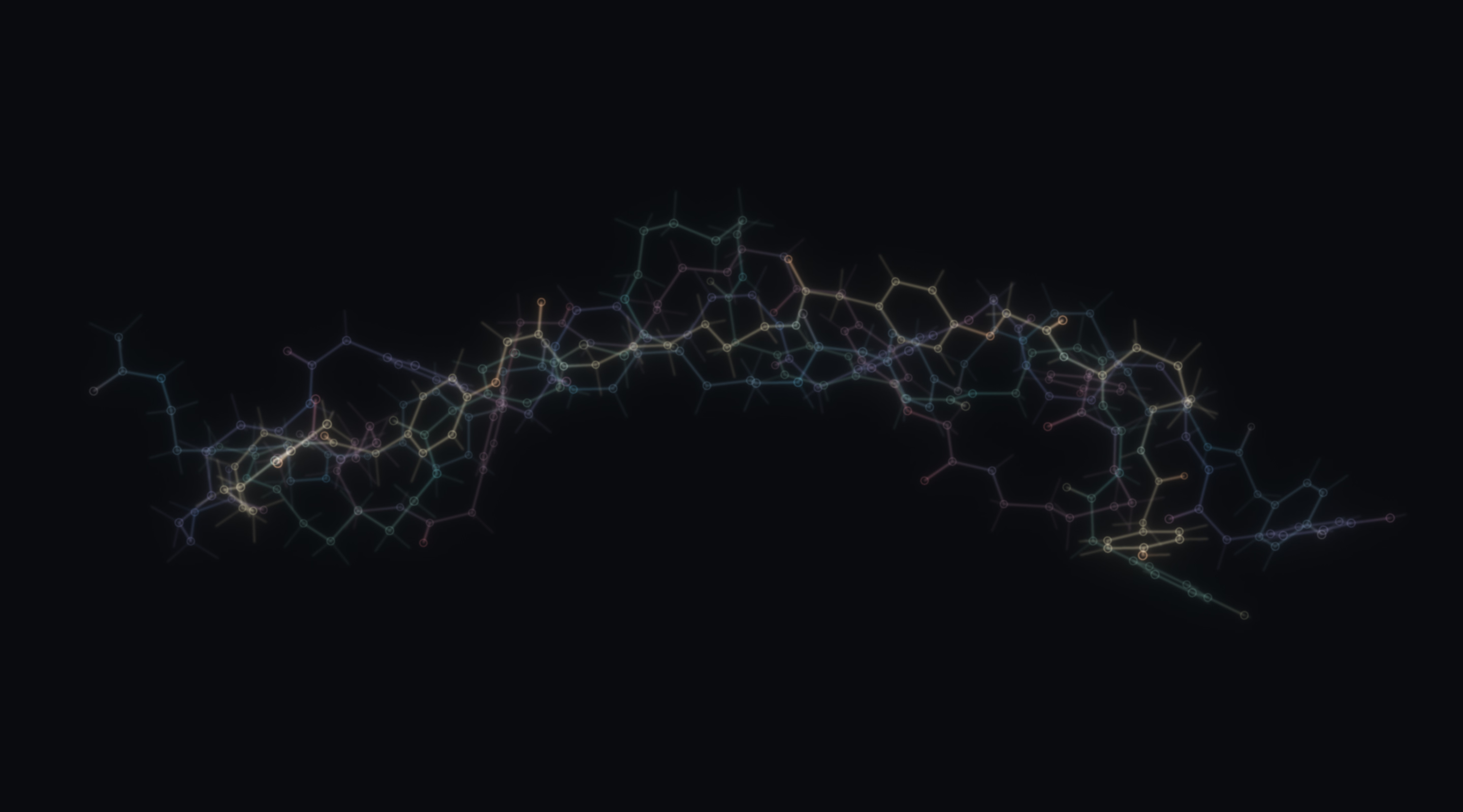
In 2025, a friend and I entered the NeurIPS Open Polymer Prediction challenge on Kaggle. The task was simple enough: given a short string of text describing one (tiny) building block of a plastic, predict five properties of the plastic itself. The time-proven and sensible entry for almost any Kaggle competition is some kind of gradient-boosted ensemble, in this case on hand-made chemical features. We wanted to see how far a 3D equivariant network could get instead, mostly because it sounded like much more fun than running endless hyperparameter tuning experiments.
What can you predict from a string?
The string is a SMILES: a molecule written as a line of text. Letters are atoms, brackets are side branches, digits close rings, and hydrogens are left out because they can be inferred. So, it’s a kind of code-language. The odd one out is the *. It is not an atom, and is instead a polymer specific thing. It marks where this unit (“monomer”) bonds to the next one when thousands of copies link up into a polymer chain.
*CC(*)c1ccccc1C(=O)OCCCCCC
* points by PolyPred's trimer builder, with the loose ends capped by hydrogen; the pink bonds are where the * were. Both drawings laid out by RDKit.The five targets are glass transition temperature, fractional free volume, thermal conductivity, density and radius of gyration. The organisers computed them by simulating the bulk polymer with molecular dynamics. There are about 8,000 monomers to learn from, and the labels are sparse: free volume has 7,030 of them, the other four between 511 and 737 each.
7,030 of 7,973 monomers have a fractional free volume label
Every square is one monomer in the training set. 7,266 of them have a single label, and none has all five.
Into 3D
An equivariant network like PaiNN (more on it in my bachelor’s thesis) reads atoms and their positions in space. A SMILES string has no positions, so they have to be made up. The cheap way, and the one PolyPred ends up using: let RDKit embed a first 3D guess, then let a force field relax it into something chemically plausible. RDKit can’t place a *, so for the embedding each one stands in as a hydrogen.
*becomes a hydrogen, RDKit's ETKDG v3 makes a first 3D guess, and the MMFF force field relaxes it. That takes 176 iterations here, and the energy readout follows the real optimiser path from 59.6 to 34.4 kcal/mol. Then the hydrogens go back to being *. The jump from the flat drawing to the first guess is drawn as a straight morph, since the embedding has no in-between steps.That is one guess. A flexible molecule has many valid shapes, called conformers, and in isolation nothing says which one it takes inside a polymer. So every molecule gets up to five, the network predicts on each, and the median is the answer.
So what is a *?
To the network, every atom is a type and a position. A polymerisation point is neither a real atom nor nothing, so it needs an answer of its own. We could keep pretending it is a hydrogen, but then the network can’t tell a chain continuing from a dead end. We could drop it, and lose where the chain goes. We gave it a type of its own, and let the network learn what it means.
- *0
- H1
- Li3
- B5
- C6
- N7
- O8
- F9
- Na11
- Si14
- P15
- S16
- Cl17
- K19
- Ca20
- Zn30
- Ge32
- Se34
- Br35
- Cd48
- Sn50
- Te52
- I53
- Pb82
*, as atomic number 0. Each type is a row in a learned embedding table, so the network works out for itself what a polymerisation point means.That still leaves where in space to put it. PolyPred has four answers. Hydrogen and carbon stand-ins are quick and know nothing about the neighbours. The more informed route builds a chain of three units, relaxes the whole thing, and cuts the middle one back out, so each * sits where the neighbouring atom actually ended up. Or skip the question and give the network the whole trimer.
Count the leaps. A string becomes a graph. The graph gets a guessed shape from a force field. One unit, in one of several shapes, stands in for a chain, and the chain for a bulk material whose properties came out of a molecular dynamics simulation. Each step is a guess, and none of them can be checked quickly. In hindsight, it is a lot to ask of a network whose whole point is taking geometry seriously. But it was for the fun of it.
How it did
We compared PaiNN against AutoGluon, an automatically tuned ensemble of tabular models on standard chemical descriptors: same molecules, same splits, 10-fold cross-validation.
- PaiNN per property
- PaiNN, all five at once
- PaiNN per property, descriptors
- PaiNN all at once, descriptors
- AutoGluon
- Hydrogen stand-in
- AutoGluon
- Whole trimer
- AutoGluon
- Borrowed from neighbours
- AutoGluon
Lower is better. Hover a row for its numbers.
The numbers as a table
| Model | Free volume (×10⁻³) | Density (×10⁻³) | Radius of gyration | Glass transition | Thermal conductivity (×10⁻³) |
|---|---|---|---|---|---|
| PaiNN per property | 4.2 ± 0.2 | 25.2 ± 4.6 | 1.49 ± 0.13 | 53.4 ± 3.9 | 25.0 ± 2.0 |
| PaiNN, all five at once | 4.4 ± 0.3 | 23.3 ± 3.8 | 1.49 ± 0.14 | 58.8 ± 4.4 | 26.9 ± 2.4 |
| PaiNN per property, descriptors | 4.2 ± 0.2 | 23.8 ± 3.4 | 1.47 ± 0.13 | 52.6 ± 4.0 | 26.0 ± 2.0 |
| PaiNN all at once, descriptors | 4.3 ± 0.2 | 22.4 ± 3.8 | 1.56 ± 0.15 | 57.1 ± 4.6 | 26.0 ± 2.0 |
| AutoGluon | 5.2 ± 0.2 | 28.2 ± 3.4 | 1.57 ± 0.14 | 52.2 ± 3.9 | 26.1 ± 2.0 |
| Model | Free volume (×10⁻³) | Density (×10⁻³) | Radius of gyration | Glass transition | Thermal conductivity (×10⁻³) |
|---|---|---|---|---|---|
| Hydrogen stand-in | 4.4 ± 0.3 | 23.1 ± 4.0 | 1.53 ± 0.11 | 56.6 ± 4.2 | 27.8 ± 2.4 |
| AutoGluon | 6.2 ± 0.3 | 33.3 ± 5.0 | 1.73 ± 0.19 | 53.4 ± 4.4 | 24.6 ± 2.6 |
| Whole trimer | 4.8 ± 0.3 | 31.5 ± 5.8 | 1.66 ± 0.19 | 60.3 ± 5.5 | 24.7 ± 3.5 |
| AutoGluon | 6.1 ± 0.3 | 35.0 ± 5.2 | 1.71 ± 0.18 | 54.0 ± 4.5 | 23.8 ± 2.4 |
| Borrowed from neighbours | 4.9 ± 0.3 | 32.0 ± 5.9 | 1.66 ± 0.18 | 59.7 ± 5.4 | 24.4 ± 3.6 |
| AutoGluon | 6.2 ± 0.3 | 33.3 ± 5.0 | 1.73 ± 0.19 | 53.4 ± 4.4 | 24.6 ± 2.6 |
Nothing earth-shattering. PaiNN matched the tuned ensemble on four properties and beat it on free volume, the one property with plenty of labels. Given all the guessing it took to get a 3D molecule in the first place, it held up better than I expected. And of all the geometries, the simplest one, the hydrogen stand-in, did best.
The package
PolyPred itself is a pip-installable Python package, built as a wheel so it would install inside Kaggle’s offline notebooks. It holds the 3D pipelines, parallelised and seeded so a cluster rebuilds the same dataset every time; PaiNN with the * type, optional descriptor injection, and single or multi-target heads with a loss that skips missing labels; conformer pooling; and grouped cross-validation with the confidence intervals of Bayle et al. (2020), shared with the baseline so the comparison is fair. The code is on GitHub.
About that leaderboard
Partway through the competition, the test set leaked, and the hosts made a new one. Our cross-validation scores were far better than anything the leaderboard showed, and we were not the only ones. The winning write-up calls its “key trick” a single line of post-processing: add 0.56 standard deviations to every glass transition prediction. It was found by probing the leaderboard rather than through any chemistry, and it would have lifted pretty much anyone’s score. We took the hint and trusted the cross-validation.