Finding gas in seismic data
Only 25 examples of the thing I had to find. Treating every column of every image as its own example turned them into more than 10,000, and small models did the rest.
- Role
- Student assistant, Ørsted
- Year
- 2024
- Stack
- Gradient boosting, Time series, Small data
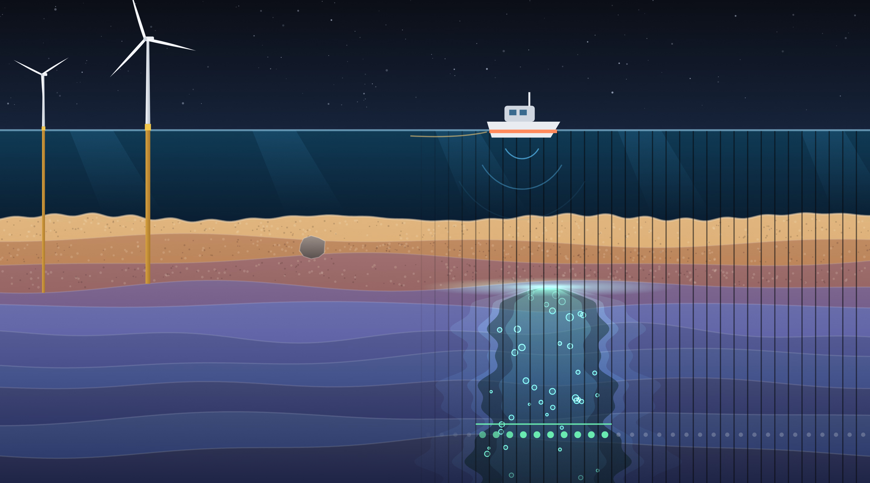
Before an offshore wind farm is built, a survey boat sails the site and maps the seabed with sound. One thing to look for is shallow gas: gas trapped in the sediment, sometimes rising in chimneys, which weakens the ground the foundations go into. In the survey images it shows up as a bright cap with a washed-out smear below it.
In summer 2024, as a student assistant in Digital Strategy at Ørsted, I worked on finding it automatically. Since I no longer work at Ørsted, I don’t actually have access to the data, so this is just a nice toy visualisation instead.
Twenty-five examples
There were a few hundred survey images. Twenty-five of them had any gas in them at all, and several of those only a sliver.
And real gas is nothing like the glowing plume in my cartoon. In an actual survey image it is a faint, washed-out patch among thousands of wiggly reflectors, noise, and other things that look a bit like it.
And that is one of the easier ones. Some chimneys are only a few columns wide, some barely dim anything, and plenty of things that are not gas look a lot like it. Not every case is easy for human eyes either.
The natural move is the one a person makes: look at the picture, draw an outline around the gas, and train a segmentation network to do the same. A chimney is a shape, and shapes are what we are good at. But 25 outlines is very little to learn a shape from, especially one that varies as much as gas does.
Turning the problem around
So I stopped asking where the outline is and asked something smaller. Take a single column of the image: one line of about 2,000 numbers, from the top of the record to the bottom. Does it pass through gas, yes or no?
To a person, one column means almost nothing. To a model, it is a signal with a clear signature: a sharp kick where the gas starts and very little below it. And every image is thousands of columns wide.
Splitting without leaking
Neighbouring columns are near copies of each other, so a careless split leaks the answer: train on one column, test on the one next to it, and anything looks brilliant. Whole images went to training, validation or test, never across. Columns at the very edge of the gas are ambiguous, so negatives were only taken a safe distance away from it, and extra columns from gas-free images kept the classes roughly balanced.
Small models
In this shape, the problem no longer needed a big model. I tried gradient boosting, small 1D convolutional networks, and wavelet and Fourier transforms followed by a classifier. The raw column worked best as input, and scikit-learn’s histogram-based gradient boosting was the most robust on so little data, with other tree models close behind. The small, simple models beat the large, complex ones.
Putting the picture back together
To read a new image: slice it into columns, classify each one, and put the answers back side by side. Column by column, the answers are a little noisy. A boulder that reflects brightly fools one column, a stray column lights up for no reason, a column in the middle of the gas gets missed.
The misses matter more than they sound. A geophysicist labels a gas zone as one continuous stretch, but the model only ever sees one column, and now and then it calls a few columns in the middle of the gas empty. A wide zone comes back as a broken row of hits. A simple smoothing filter along the line fixes both problems: it fills the holes, so the answer looks like what a geophysicist would draw, and it drops the strays. Smooth too hard, though, and a small pocket of gas vanishes with the noise. So the smoothing strength and the threshold that turns the smoothed answer into a yes or no were tuned together, like any other hyperparameters.
Put together, it worked really well.
What stuck with me
This was one of my first meetings with real-world data: small, badly unbalanced, and nothing like a textbook dataset, with a lot of brainstorming about which method could even work before any code was written. A hello world for working with real data.
The lesson that stuck is that the way people see a problem is not always the best way to hand it to a model. To us, a chimney is obviously a shape. To a model with 25 examples, it was far easier as a pile of short signals. Making the data look more alien made it much more learnable.